Picture Guide To IboView

In the 3D-View, the following controls can be used:

• Rotate View: Hold right mouse button and move mouse

• Move View: Hold left and right mouse button and move mouse

• Zoom: Hold right mouse button and turn mouse wheel

• Rotate View around cursor: Hold left and right mouse button and turn mouse wheel (holding Shift while doing this will make the movement slower)

• Select objects (atoms, orbitals): Left-click on them. Holding Shift while selecting atoms allows for selecting and de-selecting additional atoms. Right-clicking on a atom or orbital will bring up a context menu (see below).

Start IboView and load the file examples/claisen/nebpath.xyz. You should see the screen below. nebpath.xyz is a .xyz file containing 37 frames (sequential geometries) on a reaction path for the Claisen re-arrangement reaction.

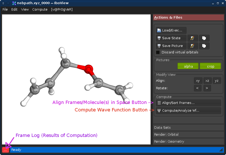
• With "Align Frames" you can align molecules in 3D space, align them to each other, remove frames, and change the order of frames (for example, to combine the two sub-paths of an IRC trace starting at a transition state). For this example this is not required.

• Pressing the "..." button will show the log of the computations performed by IboView for the current geometry frame. Since IboView has not yet performed a computation, it will be empty at this point.

• By Pressing "Compute Wave Function" or pressing Ctrl+Enter, you open a dialog offering several computation options. For now, just press OK. This will cause IboView to compute the Kohn-Sham wave functions and Intrinsic Bond Orbitals (IBOs) for the entire reaction path. This will take about 30s-2min and present the following calculation log once done (press "Close" to close it):

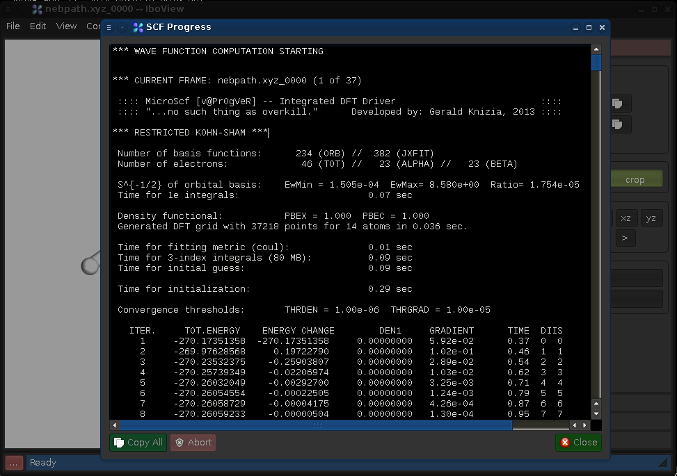
• We now have, for each frame, a set of IBOs which are an exact representation of the frame's Kohn-Sham wave function.

• Go to the tab "Data Sets", and the sub-tab "Frames". Changing either the "Current Frame" dial (left) or the frame index spinbox will move you trough the reaction path.

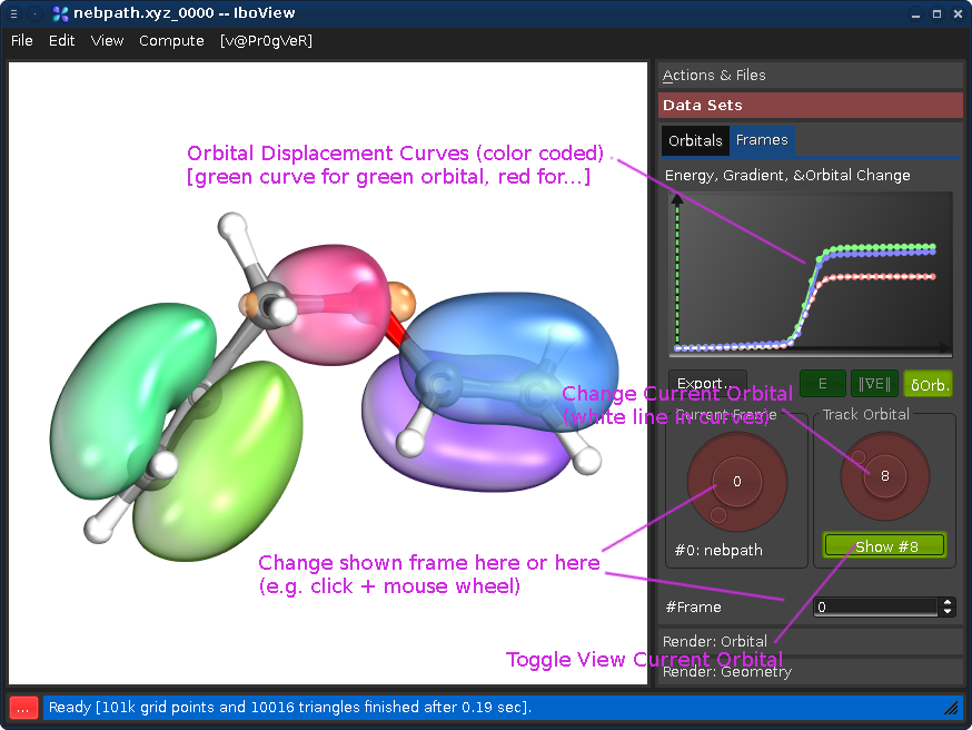
• Changing the "Track Orbital" dial (right) will show you the charge displacement curves of the current orbital ID (it is the rms deviation of the vector of the orbital's partial charges compared to the first frame). When the curve is flat, the orbital remains on the atom it started on. When it goes up, it means that the orbital moves. In the current example, there are three orbitals which do this (8, 21, and 22, all other orbitals stay where they are). Selecting them on the dial and presssing "Show #.." will render them. Once you see all three, press Ctrl+T; this will render the orbitals for all frames at once (instead of when the frame is first shown).

• If you now go through the frames, you can see how one pi-bond becomes a sigma bond, a sigma bond a pi bond, and one pi bond moves---in full agreement with the classical curly arrow mechanism.

• The theory behind this and the correspondence to curly arrows was developed in:

  G Knizia and JEMN Klein; Electron flow in reaction mechanisms---revealed from first principles Angew. Chem. Int. Ed. 54, 5518 (2015) DOI: 10.1002/anie.201410637

  It is a short read, we recommend looking into it to get the most out of IboView.

• IboView can be used as a mundane orbital visualization program. It has an own orbital grid kernel and does not need cube files. Instead, orbital coefficients and basis declarations are imported from quantum chemistry software.

• Using with Molpro 2012: A simple complete input is the following:

  memory,200,m;
  
  geometry={
    B          0.877457      -0.000000      -0.000000
    B         -0.877457      -0.000000       0.000000
    H         -0.000001       0.000002       0.972827
    H         -0.000001       0.000002      -0.972827
    H         -1.448973      -1.038057      -0.000000
    H         -1.448974       1.038056      -0.000000
    H          1.448973      -1.038057       0.000000
    H          1.448975       1.038055       0.000000
  }
  
  basis=tzvpp
  {df-rks,pbe}
  {put,xml,b2h6.xml; nosort}
  

  The last command, {put.xml,filename.xml; nosort} exports the last orbital set to the given xml file name. This xml file can then be loaded with IboView. Orbital specifications can be given as usual on the card (e.g., for MCSCF natural orbitals or similar).

• Using with Turbomole: Run your calculation as usual and export it via Turbomole's tm2molden program into .molden file format. The .molden file can then be read with IboView.

  If only .xyz files are required, use Tubomole's t2x program to export a .xyz file (with gradient information). This can be used to visualize geometry optimization progress, for example.

• Using with Orca: Use "orca_2mkl -molden" to generate a file called basename.molden.input from the basename.gbw file. This generated molden file can be read by IboView.

• Using with Molcas: .molden files generated by Molcas can be read by IboView.

• Using with Gaussian: Use route card #P GFINPUT IOP(6/7=3) in the input to export a Molden file. A complete example input is:

  %nprocshared=4
  %mem=8GB
  %chk=butadiene.chk
  #p gfinput IOP(6/7=3) b3lyp/Def2TZVP geom=connectivity
  
  Dummy title of calculation
  
  0 1
  C                  0.60183500    1.75151100    0.00000000
  H                 -0.32531400    2.32078200    0.00000000
  H                  1.52430700    2.32419400    0.00000000
  C                  0.60183500    0.41095800    0.00000000
  H                  1.55162000   -0.12489300    0.00000000
  C                 -0.60183500   -0.41095800    0.00000000
  H                 -1.55162000    0.12489300    0.00000000
  C                 -0.60183500   -1.75151100    0.00000000
  H                  0.32531400   -2.32078200    0.00000000
  H                 -1.52430700   -2.32419400    0.00000000
  

  Notes:

  • Final newline is important.

  • 6-31G-family basis sets are not supported, since IboView does not support "shared sp" shells of basis functions. Please use other basis sets (e.g., def2-TZVP/def2-TZVPP) instead of the 6-31G family of basis sets.

  • This works only with single point calculations. If used in compound jobs including geometry optimizations or frequency calculations, output will be garbled. Please split inputs accordingly.

  • See also: http://www.cmbi.ru.nl/molden/gauss.html for additional comments on getting .molden files from Gaussian.

• Double-Click an orbital in the Data Set tab to render it. Various visualization options can be changed under Render: Orbitals/Surfaces:

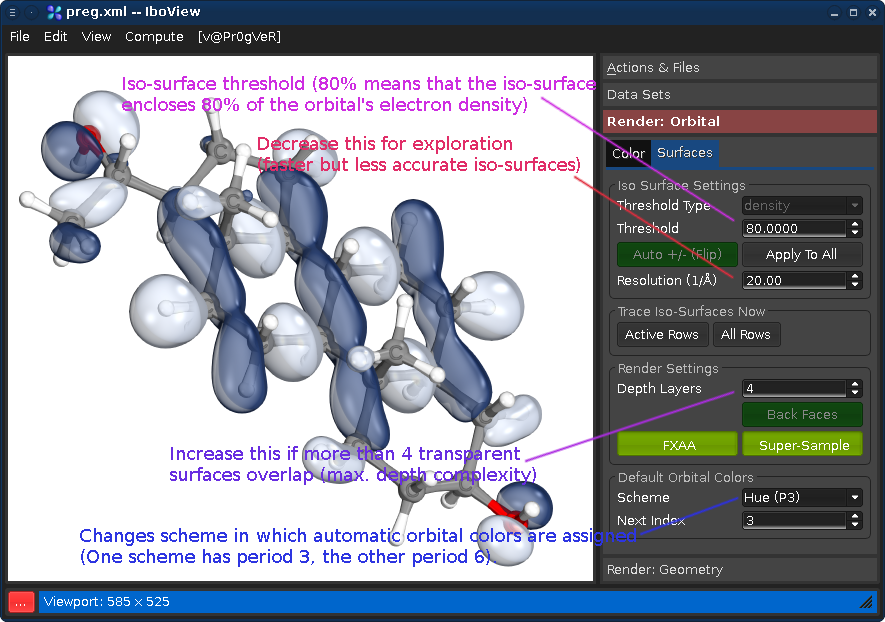
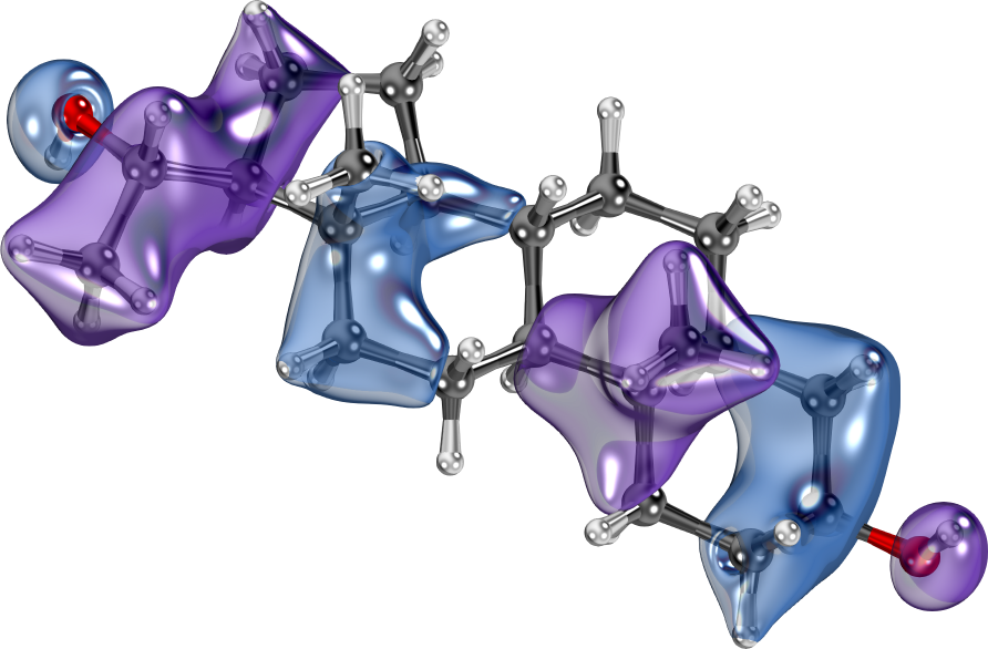
• Note: The default resolution of 20 pt/A is recommended for publication purposes, but is much higher than other programs use. For exploration purposes, a smaller resolution is sufficient, especially for very delocalized orbitals. Doubling this value will multiply iso-trace time by factor 8 (3rd order scaling).

• We are commited to making quantum chemistry more shiny! The first person who uses IboView's super-shiny mode in an actual publication (and cites the curly arrow paper) will receive my personal Friends Of Shininess award! 8]

• IboView can currently not compute open-shell or pseudo-potential wavefunctions by itself, but it can import them from Molpro or Turbomole and perform an IBO analysis on them.

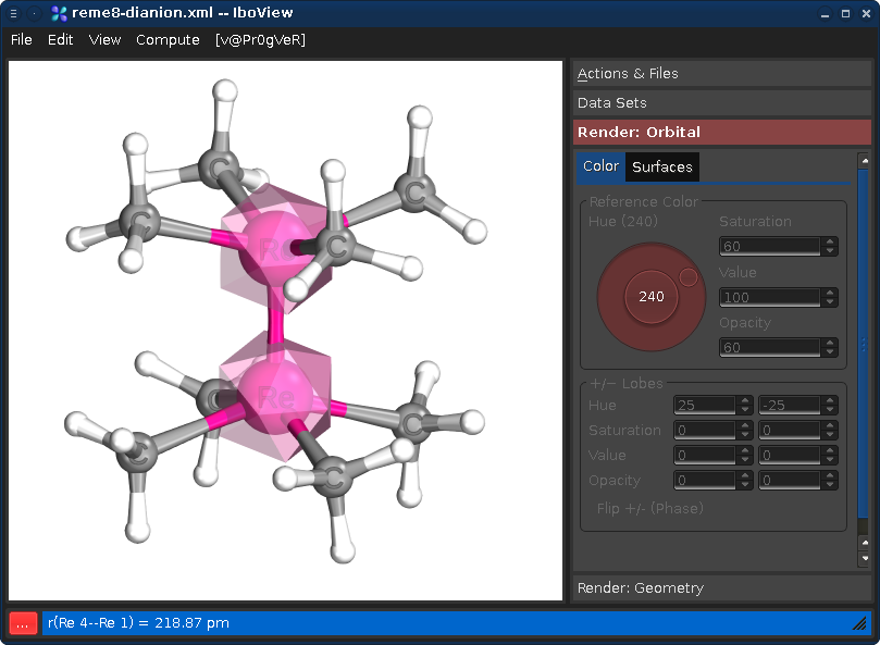
• To this end, load the exported result .xml or .molden file as described in the last section. Then Press Ctrl+Enter and run a chemical analysis only (no Kohn-Sham). This will compute partial charges and IBOs (see: G. Knizia, Intrinsic atomic orbitals: An unbiased bridge between quantum theory and chemical concepts J. Chem. Theory Comput., 9 4834 (2013))

• Let us take the file re2me8-dianion.xml from the example directory. Assume we wanted to know which orbitals are localized to the two rhenium centers. Select the two Rhenium atoms (left-click one, then hold shift and left-click the other). You see the following:

• Now right-click on one of the selected atoms, and choose "Find Orbitals..." This will bring up the following dialog, showing all orbitals which have significant contributions on the center:

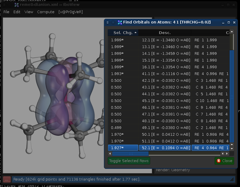
• The first column shows the accumulated charge the orbital has on the selected centers, the second column its designation, and the third (not shown here) the orbital partial charges. Here we would see a total of four orbitals which have their charge evenly split between the two Re centers (orbitals 41.1, 50.1, 51.1, and 52.2). Thus, there is a quadruple bond.

• The orbitals can be rendered by double-clicking on them in the Find Orbitals dialog. Afterwards the dialog can be closed.

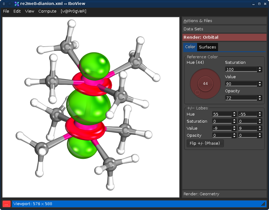
• Orbitals can be colored to your's heart's content

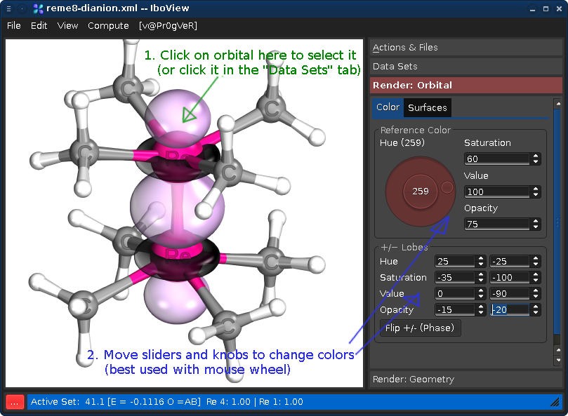
• Beware: Some color combinations are more tasteful than others...

• ...can be found in the README.txt file distributed with the program, including a number of usability and interfacing hints.

• A gallery of various common bond types will be presented on the main page soon.